As AI models are deployed in production, they face an ever-changing data landscape that can lead to a phenomenon known as data drift. Data drift occurs when the statistical properties of the data used to train a model start to diverge from the data the model encounters during inference. This can lead to a degradation in model performance over time, as the model’s learned patterns and relationships no longer accurately reflect the real-world data.

Detecting data drift is a critical task for ML engineers and data scientists tasked with maintaining the health and reliability of AI systems. By proactively identifying data drift, teams can take corrective action to retrain, fine-tune or rebuild models before production performance suffers.

In this blog post, we’ll explore 5 powerful methods for detecting data drift, complete with real-world examples and code samples. Whether you’re new to the topic of model monitoring or a seasoned AI expert, these techniques will equip you with the tools needed to keep your AI systems robust and up-to-date.

1. Distribution Divergence Metrics

One of the most common and intuitive approaches to detecting data drift is to compare the statistical distributions of the training data and production data. If these distributions begin to significantly diverge, it’s a clear sign that data drift is occurring.

A popular metric for quantifying distribution divergence is the Kullback-Leibler (KL) Divergence. The KL Divergence measures the difference between two probability distributions P and Q, and is defined as:

Where P represents the training data distribution and Q represents the production data distribution.

As an example, let’s say we’re monitoring a image classification model that categorizes different types of flowers. We can track the KL Divergence between the RGB color distributions of the training flowers versus the production flowers over time. If we start to see the KL Divergence steadily increase, it’s a signal that the color properties of the production flower images are drifting away from the training data, which could negatively impact the model’s ability to accurately classify new flowers.

Here’s some sample Python code using the Scipy library to calculate KL Divergence:

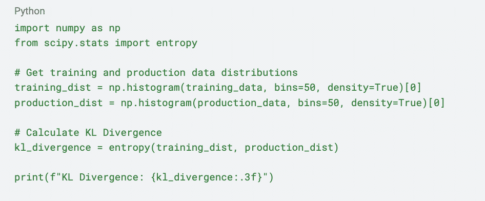
The KL Divergence is just one example of a distribution divergence metric. Other common options include Jensen-Shannon Divergence, Wasserstein Distance, and Maximum Mean Discrepancy. The best metric to use will depend on the specific characteristics of your data and model.

2. Feature Drift Analysis

Rather than looking at overall data distribution shifts, we can also analyze the drift occurring at the individual feature level. This is particularly useful when dealing with high-dimensional data, where overall distribution changes may mask more subtle drifts happening in specific input features.

One effective technique is to calculate feature importance/correlation metrics on the training data, and then monitor for changes in these metrics on the production data. For example, assuming a linear relationship, we could track the Pearson correlation coefficient between each feature and the target variable. If we start to see certain features becoming more or less correlated with the target over time, it indicates those features may be drifting.

Let’s look at an example using a tabular dataset of customer transactions. We’ll calculate the Pearson correlation of each feature to the target variable (whether the customer made a purchase) on the training data, then monitor for changes in those correlations on the production data:

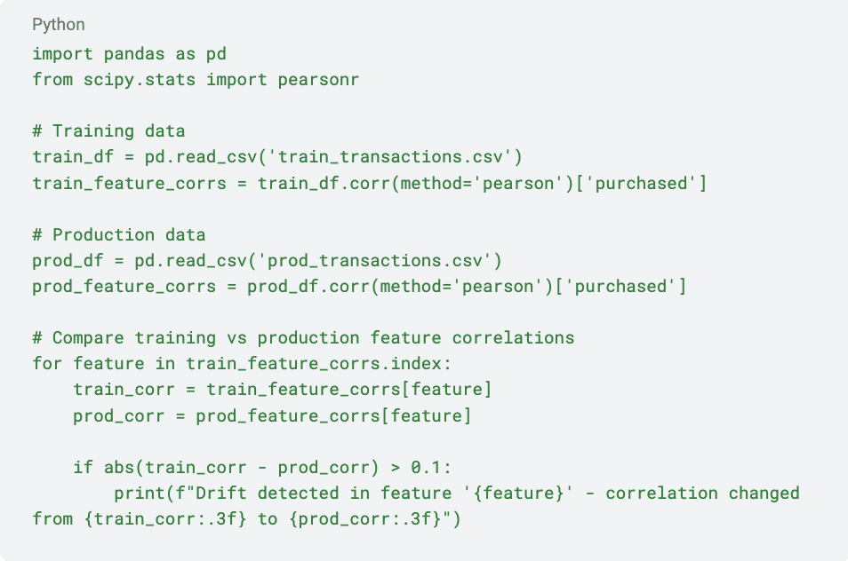
In this example, we flag any features where the Pearson correlation to the target variable has changed by more than 0.1 between the training and production datasets. Monitoring these feature-level drifts can provide valuable insights into which parts of the data are changing over time.

3. Anomaly Detection

Another useful technique for identifying data drift is to leverage anomaly detection methods. The core idea is to build a model that can identify “outlier” data points that deviate significantly from the training data distribution. An increase in the number of anomalous data points in production is a clear sign of data drift.

One popular anomaly detection approach is Isolation Forests. Isolation Forests work by randomly partitioning the feature space and identifying data points that are more “isolated” from the rest of the distribution. Points that require fewer partitions to isolate are considered anomalies.

Let’s see how we can use Isolation Forests to detect data drift in our flower classification example:

In this example, we first train an Isolation Forest model on the training data. We then apply that model to the production data and monitor the percentage of data points flagged as anomalies. If this anomaly rate starts to significantly exceed the 1% rate we saw in training, it’s a clear sign that the production data distribution has drifted from the training distribution.

Anomaly detection is a powerful tool, but it’s important to carefully tune the hyperparameters (like the contamination rate) to ensure you’re accurately capturing genuine distribution shifts rather than just detecting normal noise in the data.

4. Segment-based Drift Analysis

Rather than looking at the data distribution as a whole, another effective technique is to analyze drift on specific data segments or subgroups. This is particularly useful when your production data contains distinct cohorts or populations that may be drifting at different rates.

The general approach is to first define the relevant data segments (e.g. by customer geography, product type, user demographics, etc.). Then, you can apply the distribution divergence and anomaly detection methods we discussed earlier, but do the analysis independently on each data segment.

By monitoring drift at the segment level, you can identify which parts of your data are most prone to change, and focus your model maintenance efforts accordingly. This granular view can provide much more actionable insights than simply looking at the overall data distribution.

Here’s some sample code using pandas to implement segment-based drift analysis:

By breaking down the analysis at the segment level, you can get a much more granular and actionable understanding of where data drift is occurring in your production environment. This can inform targeted model updates and retraining strategies to maintain performance across diverse data subgroups.

5. Adversarial Validation

The final technique we’ll cover is adversarial validation – a method that can simultaneously detect both data distribution drift and concept drift.

The core idea behind adversarial validation is to train a binary classifier to distinguish between the training data and production data. If the training and production data are truly independent and identically distributed (i.i.d.), this classification task should be very difficult, with the model performing only slightly better than random guessing.

However, if there are significant differences between the training and production data distributions, the adversarial model should be able to learn meaningful patterns to discriminate between the two datasets. The better the adversarial model performs, the stronger the evidence of data drift.

Furthermore, if the adversarial model performs well even after controlling for distribution shifts (e.g. by applying techniques like feature importance analysis), it indicates the presence of concept drift – changes in the underlying relationships between inputs and outputs.

Here’s some sample code using scikit-learn to implement adversarial validation:

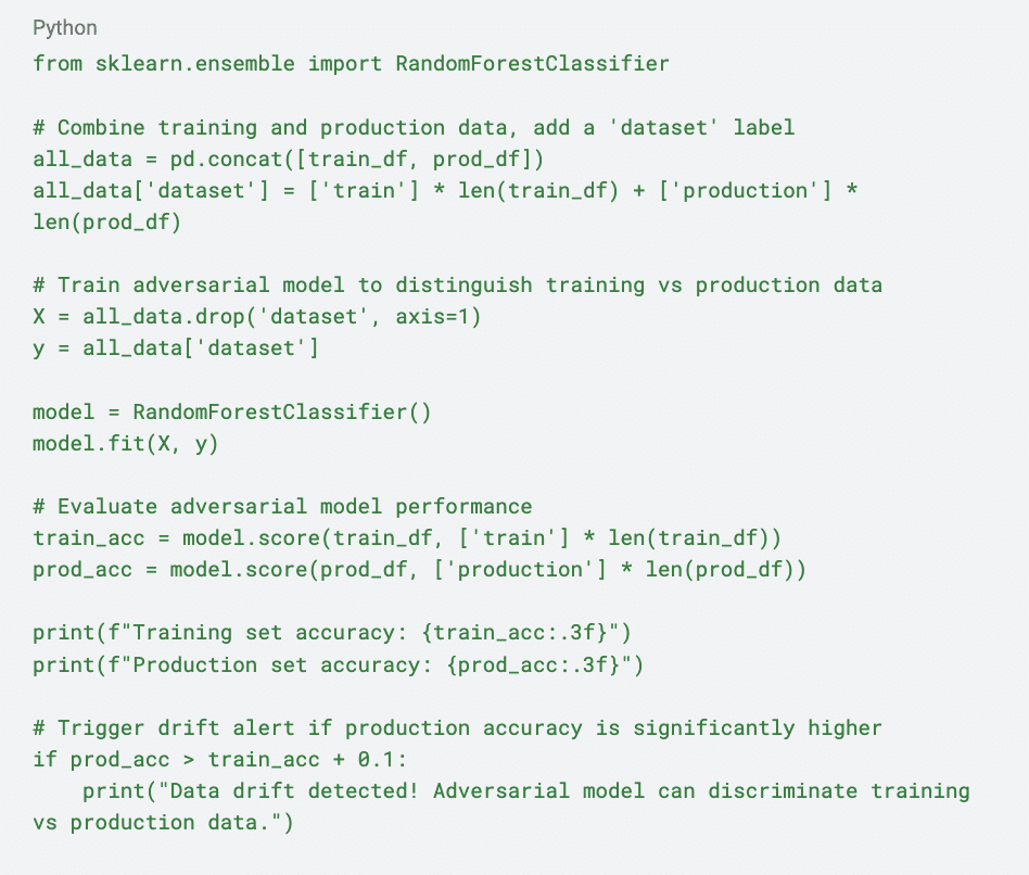
In this example, we first combine the training and production datasets, adding a ‘dataset’ label to indicate the source. We then train a Random Forest classifier to predict the dataset label based on the feature values.

If the training and production data are truly i.i.d., we’d expect the adversarial model to perform only slightly better than 50% accuracy on both sets. However, if the model can achieve significantly higher accuracy on the production data, it’s a clear sign that the two datasets have diverged in meaningful ways.

Adversarial validation is a powerful and versatile technique that can uncover both distribution shifts and concept drift. By training a model to discriminate between training and production data, we can get a holistic view of how an AI system’s data landscape is evolving over time.

Conclusion

Detecting data drift is a crucial capability for maintaining the long-term health and reliability of AI systems. In this blog post, we’ve explored 5 proven techniques for identifying data drift:

• Distribution Divergence Metrics: Comparing the statistical properties of training and production data distributions.
• Feature Drift Analysis: Monitoring changes in feature importance and correlations over time.
• Anomaly Detection: Identifying outliers in production data that diverge from the training distribution.
• Segment-based Drift Analysis: Monitoring drift patterns across different data subgroups and populations.
• Adversarial Validation: Training a classifier to distinguish training and production data as a proxy for overall drift.

Each of these methods provides a unique perspective on data drift, and combining them can give you a comprehensive view of how your AI system’s data is evolving. By proactively detecting and addressing data drift, you can ensure your models remain accurate, reliable, and responsive to the changing real-world environment.

A proactive approach to data drift involves not only preventive measures but also continuous monitoring tools to anticipate and mitigate data drift. The Radicalbit AI Monitoring Open Source platform offers a comprehensive suite of tools to proactively detect and mitigate data drift, maximizing model performance.

Learn more about the platform on the GitHub Page!